Introduction
Sales forecasting is a pivotal process for companies aiming to strategically plan their future business operations. Accurate sales forecasting empowers businesses to make data-driven decisions regarding inventory management, production planning, marketing campaigns, and staffing. This project focuses on predicting the future sales of a company’s products or services over a specified period by leveraging historical sales data, identifying trends, and employing statistical models for predictions.
Importance of Sales Forecasting:
Sales forecasting plays a vital role in business success for several reasons:
- Inventory Management: Precise sales forecasts aid in avoiding stockouts or overstocking, mitigating lost sales and excessive costs.
- Production Planning: Sales forecasts assist companies in planning production activities according to expected demand, ensuring efficient resource allocation and minimizing waste.
- Supply Ordering: Accurate forecasts are crucial in ordering supplies to meet customer demand. Overestimating demand leads to bloated inventory and increased costs, while underestimating demand results in unmet customer needs.
- Marketing Campaigns: Sales forecasts inform the development and execution of targeted marketing campaigns aligned with future sales objectives.
- Financial Planning: Sales forecasts serve as a foundation for revenue projections, budgeting, and cash flow management, aiding in effective financial planning.
Overall, a robust sales forecasting project empowers companies to make strategic decisions, enhancing efficiency, profitability, and competitiveness in the market.
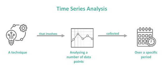
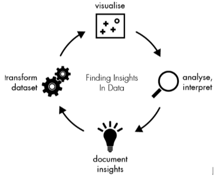
Exploratory Data Analysis
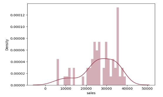
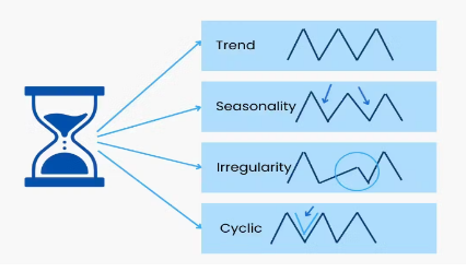
Exploratory Data Analysis (EDA) for time series involves examining the characteristics and patterns within a sequential dataset over time. Key steps include assessing stationarity, identifying seasonality, and understanding autocorrelation. By visualizing data plots and conducting statistical tests, analysts can gain insights into the underlying structure of the time series, informing subsequent modelling and forecasting efforts.
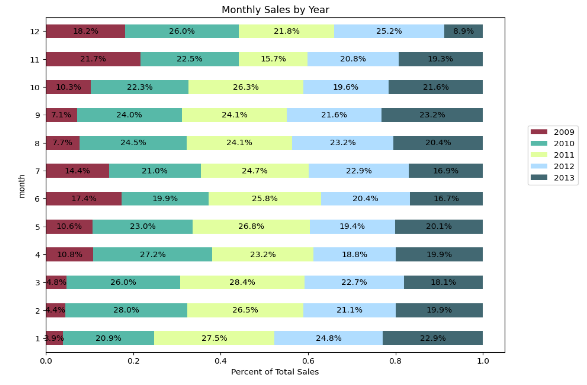
Additive vs. Multiplicative Check:
- Additive: When the seasonal fluctuations in the data are roughly constant in size over time.
- Multiplicative: When the seasonal fluctuations in the data change proportionally to the level of the data
- You can perform a visual inspection of the data or calculate the ratio of seasonal variation to the mean to determine whether the data exhibits additive or multiplicative seasonality.
Stationarity Check:
- A time series is said to be stationary if its statistical properties such as mean, variance, and autocorrelation remain constant over time.
- You can use statistical tests like the Augmented Dickey-Fuller (ADF) test or the Kwiatkowski-Phillips-Schmidt-Shin (KPSS) test to check for stationarity.
Differencing Technique – Non-Seasonal:
- If the time series is not stationary, you can apply differencing to make it stationary.
- Take the first difference by subtracting each value from its previous value.
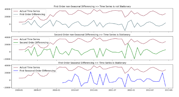
Differencing Technique – Seasonal:
- If the data exhibits seasonal patterns, seasonal differencing may be necessary.
- Take the difference between an observation and the observation at the previous season.
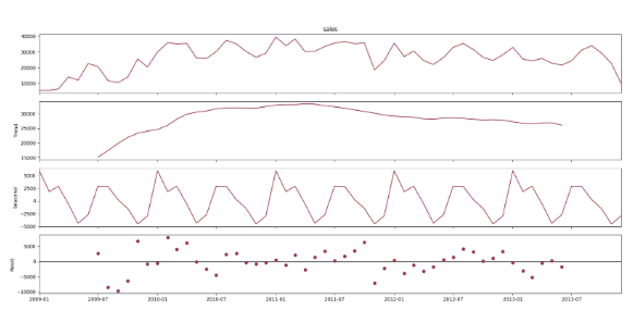
Stationarity and Differencing Technique Results Plots:
- Plot the time series data before and after applying differencing techniques to visualize.
- Also, plot the autocorrelation function (ACF) and partial autocorrelation function (PACF) plots to identify any remaining autocorrelation.
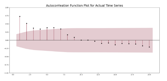
Autocorrelation Function Plot for Actual Time Series:
- Plot the ACF to visualize the correlation between a time series and its lagged values.
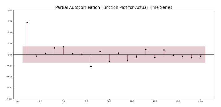
Partial Autocorrelation Function Plot for Actual Time Series:
- Plot the PACF to visualize the correlation between a time series and its lagged values after removing the effects of intermediate lags.
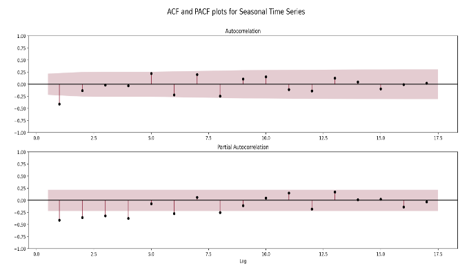
ACF and PACF Plots for Seasonal Time Series:
- Plot the ACF and PACF for the seasonally differenced time series to identify the seasonal components in the data.
Models & Prediction
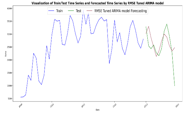
ARIMA RMSE Tuned Model:
This refers to an ARIMA (Autoregressive Integrated Moving Average) model where the parameters have been tuned to minimize the Root Mean Squared Error (RMSE) on a validation dataset. ARIMA is a popular time series forecasting model that incorporates autoregression, differencing, and moving average components.

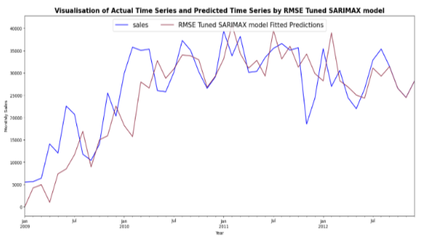
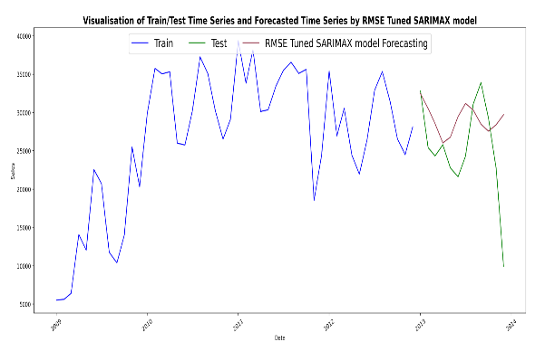
SARIMAX RMSE Tuned Model:
Similar to ARIMA, SARIMAX (Seasonal Autoregressive Integrated Moving Average with exogenous regressors) is a time series forecasting model that includes seasonal components and can also handle exogenous variables. This model has been tuned to minimize RMSE.
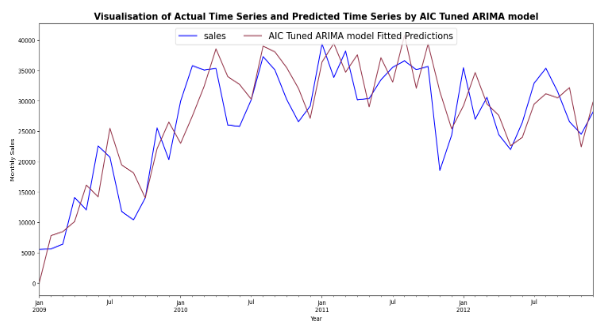
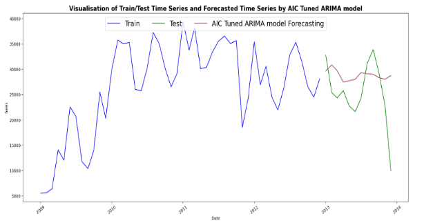
ARIMA AIC Tuned Model:
In this case, the ARIMA model’s parameters have been selected to minimize the Akaike Information Criterion (AIC), which is a measure of the model’s goodness of fit while penalizing for the number of parameters used.
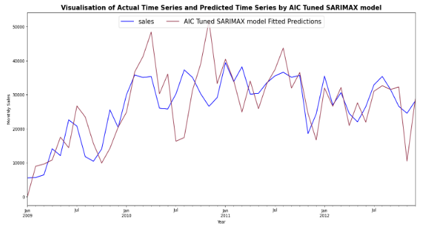
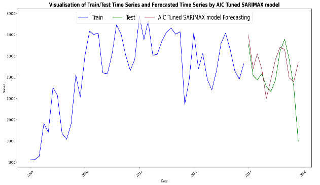
SARIMAX AIC Tuned Model:
Similar to the ARIMA AIC Tuned Model, this refers to a SARIMAX model where the parameters have been selected to minimize the AIC.
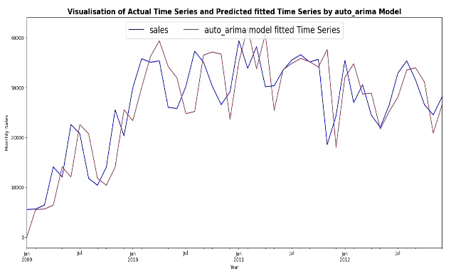
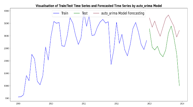
Auto ARIMA Hyperparameter Tuning:
Auto ARIMA is a method for automatically selecting the optimal combination of ARIMA parameters (p, d, q) and seasonal parameters (P, D, Q, m) based on minimizing a chosen metric such as AIC or BIC (Bayesian Information Criterion).
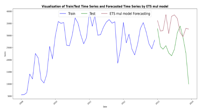
Exponential Smoothing (ETS) Model:
Exponential Smoothing is a time series forecasting method that assigns exponentially decreasing weights to past observations. This model can be tuned using various parameters to optimize its performance.
Best results & Conclusion
while the ARIMA model showed promising results on the test dataset, it’s crucial to conduct a thorough analysis of our case data and compare the performance of multiple forecasting models before selecting the most appropriate one for our specific business needs.
To facilitate this process, we will examine various aspects such as the nature and patterns of our sales data, seasonal trends, any underlying dependencies or correlations, and the complexity of the dataset. Additionally, we will assess the strengths and limitations of each forecasting model, considering factors such as computational efficiency, ease of implementation, interpretability, and the ability to handle specific characteristics of our data.
By conducting a comprehensive analysis and comparison, we can identify the forecasting model that best aligns with the unique requirements and dynamics of our business. This approach ensures that our selected model not only demonstrates superior performance on the test dataset but also effectively captures the nuances of our sales data, enabling us to make accurate predictions and informed strategic decisions.
Ultimately, through diligent analysis and evaluation, we can confidently choose the most suitable forecasting model to drive our business forward and achieve our desired objectives with precision and reliability.